

‘Bloom’ing Efficient Filter
Bloom filters are named for their creator, Burton Howard Bloom. They have nothing to do with plants.
November 10th, 2019
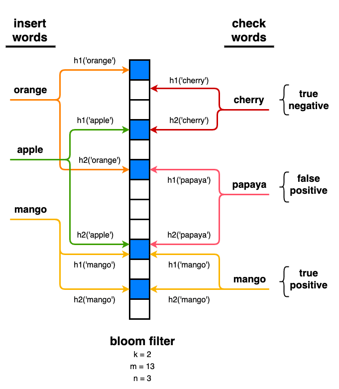
A bloom filter is a probabilistic data structure. It’s used to quickly exclude obviously irrelevant information in exchange for tolerating some false positives. A bloom filter can say “this item definitely does not belong”, or “this item might belong, but it might not”. The best part is that the false alarm positive can be calculated and controlled.
Bloom filters function a lot like a hash table, but they use memory much more efficiently. A bloom filter uses less memory because it doesn’t deal with collisions, so it has no need to store the actual item. In fact, all we need is one bit to store true or false. This means that a bloom filter can be computed once, stored in a compact bitmap, and loaded on startup or as needed.
A hash table requires 4 or 8 bytes per index while a bloom filter only requires one bit.
To check if an item is in the desired set, simply hash it and check the corresponding bit in the bitmap. If the bit is set to 0, there’s no way this item is in the desired set. If the bit is set to 1, this item might be in the desired set or it might be a collision, e.g. two items that hash to the same value. Bloom Filters by Example allows you to create and play with your own filter.
If you’re familiar with handling collisions in a hash table, you’re aware that multiple items (e.g. words) can hash to the same value. We try to avoid this by using a larger hash table, but some collisions will happen no matter what. In a bloom filter, we use the number of hash functions and the size of the filter to control the desired false positive rate.
Project Setup
The first step of a designing a good experiment is to identify a test case and declare an expected outcome. Let’s find a large text file, and count a specific set of words. I would expect this to be faster than counting all words.
I’m intentionally not verifying set inclusion with this application. I want the false positives to be reported at the end; we’re going to measure the actual false positive rate and compare it to the rate predicted by the filter design. In practice the application would double check inclusion before reporting.
Let’s start by downloading a text version of Alice in Wonderland from Project Gutenberg for testing. For fun, we’ll count occurrences of seven words commonly associated with Alice in Wonderland: alice, cake, cat, hatter, rabbit, queen, tea. Let’s add computer, bringing the total number of words to eight.
We’ll see some surprising words in the results (such as computer) because of the Project Gutenberg license in the text file.
Generate Bloom Filters
Now we can set the filter size based on a desired false positive rate. This is an experiment, so we’ll make two filters: one with ~10% probability and one with ~1% probability of false positives. To keep things simple, we can use one hash function (a Java built-in). Probability of false positives, P(FP), is approximately:
- k hash functions used
- m total bits in the filter
- n items inserted (sometimes you’ll have to guess n)
Using more hash functions allows you to use less memory without increasing false postives, but it also requires more computations and can slow down the application.
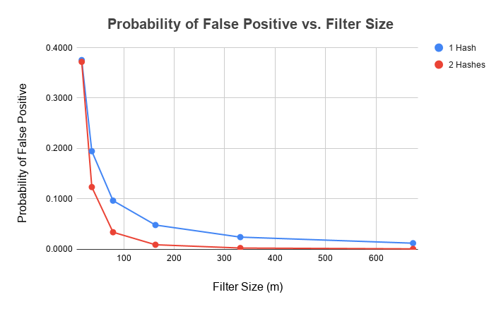
From the plot, if we want a 10% P(FP), we need a filter with 79 bits. We increase the filter size to 673 bits for a 1% P(FP). We have a few options for storing the filters on disk. We can save the raw bitmap in a binary file which would be very compact but not easily interpreted or verified. Instead, let’s save only the bits (indices) with a 1 or true. It’s still compact, but it’s much easier to inspect and understand.
Indices for 79 filter size:
[67, 75, 20, 18, 65, 53, 55, 67]

Indices for 673 filter size:
[101, 294, 619, 579, 4, 409, 611, 42]
We can already see the effects of the probabilistic nature of our bloom filter. The smaller filter (10% probability of false positives) has two words map to the same filter index. Since we populated our filter with eight words, we could expect 0.1 probability * 8 = 0.8 words to overlap (a probability of false alarm is actually the probability that unique words map to the same index). The larger filter has 8 total bits set, as expected.
Notice, the number of bits in a filter isn’t divisible by eight. Hash tables typically use a prime number for table size. We’ll waste a few bytes, but it will be a small fraction of the total filter size in practice.
Add Bloom Filter to Mapper
Start by creating a Filter class. We can leverage Java’s BitSet for the bitmap. Given a desired filter size, create a bitmap with the necessary number of bits. Then, read filter indices from disk and set them to 1.
import java.util.BitSet;
private static class Filter{
  BitSet filter;
  int filterSize = 0;
  Filter(String filterFile) throws NumberFormatException, IOException{

    //open filter file and create filter
    File file = new File(filterFile);
    BufferedReader br = new BufferedReader(new FileReader(file));

    // create bitmap
    filterSize = Integer.valueOf(br.readLine());
    filter = new BitSet(filterSize);

    // for each marked element in filter, update bitmap
    String s;
    while((s = br.readLine()) != null) {
      filter.set(Integer.valueOf(s));
    }

    br.close();
  }

  boolean isSet(int bit) {
    return filter.get(bit);
  }

  int getIndex(String word) {
    int index = word.hashCode()%filterSize;
    if(index < 0) {
      index += filterSize;
    }

    return index;
  }
}
Using an existing MapReduce word count application as a starting point, add an optional bloom filter to the Mapper step. Our updated mapper looks like this:
// print word + "1" for counting
public Mapper(String line, Filter filter) // filter may be null
{
  String[] tokens = line.split(" ");
  for(String temp: tokens)
  {
    temp = temp.toLowerCase();

    if(filter == null || filter.isSet(filter.getIndex(temp))){
      temp += " 1";
      stringList.add(temp);
    }
  }
}
Measure Performance
Generate a Baseline
Let’s do a full word count on Alice in Wonderland without any code changes or filtering. This will establish a baseline for comparing runtimes and allow us to compute an accurate false positive rate (number of false positives divided by the total number of unique words). Using our existing word counter:
$ time script/driver.sh alice_in_wonderland.txt 778 # count everything
real	0m0.719s
user	0m3.713s # amount of time spent by CPUs
sys	0m0.772s
It took our word counter about 3.7 seconds to tally ~3,000 unique words. Some of the results indicate we could improve our filtering, but it’s ok for now. Let’s look at some of the word counts (remember, the Gutenberg License is in our text file).
$ sort -k 1 reduce_results.all.txt | tail -10
yet 25
you 481
young 5
your 71
yours 3
yourself 10
youth 6
zealand 1
zigzag 1
zip 1
Test with ~10% Probability of False Positives
Using the smaller filter size, run the word counter again. Is it faster? How many extra words are reported?
$ time script/driver.sh alice_in_wonderland.txt 778 bloom_filter.79.txt
real	0m0.634s
user	0m3.414s # CPU time
sys	0m0.786s

$ cat reduce_results.79.txt | wc -l
     286 # this is about 10% of 3k unique words
Unexpectedly, the word counter with a filter only takes 0.3 seconds less CPU time. This is why it’s a good idea to identify an application’s bottlenecks before optimizing it. I suspect most of the processing time is spent in the Splitter, Stemmer, and Mapper and is unaffected by filtering. Since the goal is to have some fun experimenting with bloom filters, I’m curious but not worried about timing results.
Test with ~ 1% Probability of False Positives
Rerun the word counter with the larger filter (673 bits with 1% false positives).
$ time script/driver.sh alice_in_wonderland.txt 778 bloom_filter.673.txt
real	0m0.588s
user	0m3.324s # CPU time
sys	0m0.747s

$ cat reduce_results.673.txt | wc -l
      36 # about 1% of 3k unique words
Using a larger filter, with smaller false positive probability, reduced timing a little more. More importantly, it greatly reduced the number of reported results.
All counted words (filter words in bold):
- alice 403
- because 16
- binary 1
- books 2
- cake 3
- cat 37
- computer 2
- different 10
- directions 3
- draggled 1
- e 29
- end 20
- fallen 4
- fifteen 1
- fortunately 1
- hatter 56
- held 4
- hiss 1
- jaw 1
- kind 8
- kiss 1
- learned 1
- leave 9
- never 48
- order 3
- out 118
- queen 75
- rabbit 51
- say 51
- sends 1
- solid 1
- speed 1
- strange 5
- tea 19
- top 8
- water 5
Not all words are counted. You might be wondering if that means our count is wrong for some words. Since a hash function is deterministic (gives the same output with consistent input), a word will either always or never pass through the filter - until we load a new filter.
In a production application, we would check for inclusion in our list of words before printing results (probably at the Reducer level). I skipped that step here so we could see what it really means to have a false positive rate. In the end, the filter reduced timing by 0.5 seconds or 13%. It’s not a huge improvement, but then again it didn’t take much effort to implement.
Because our list of words is so small, we’d be better off using a traditional set and having zero probability of false positives. The difference in memory usage would be negligible and our output would only include the words of interest. Coding it up would also be simpler with a built-in set.